Note
Go to the end to download the full example code.
Reading a radial filament from its file#
A collimated 800 nm, 30 fs beam of 300 µm waist and 0.88 mJ in 1 bar of argon, about
three times the critical power: it collapses, the plasma arrests the collapse, and a
filament forms. The run is a plain prop_radial(), every
argument an object a recipe writes as a table, and it is the call the filament’s example
recipe mirrors (Recipe.example("filament")). The lesson
A radial filament in argon explains the physics; this page shows what
a radial file can be asked for afterwards: the beam’s characteristic numbers, its
spectrum across the beam and on the axis, and its far field. Each reader takes only the
file.
from time import perf_counter

import matplotlib.pyplot as plt
import numpy as np

from solprop.driver import SimulationSettings, prop_radial
from solprop.grid import EnvelopeGrid, RadialGrid
from solprop.nonlinear.envelope_plasma import EnvelopePlasmaResponse
from solprop.nonlinear.optmat_rates import OptmatRate
from solprop.nonlinear.responses import KerrResponse
from solprop.physdata import gamma3
from solprop.processing import far_field, on_axis_spectra, radial_spectrum
from solprop.pulses import GaussianPulse, SpatialPulse
from solprop.spatial import SpatialMedium
from solprop.stats import StatsSpec
from solprop.stepper import PIController
from solprop.tools import beam_params, pulse_peak_power

started = perf_counter()
The run#
The radial grid reaches four waists; the envelope grid leaves out the third harmonic.
length = 0.25
grid = EnvelopeGrid.from_limits(length, 800e-9, (500e-9, 1.4e-6), 300e-15, thg=False)
space = RadialGrid(1.2e-3, 128)
settings = SimulationSettings(
    controller=PIController(rtol=1e-5, atol=1e-11),
    # Every 3.125 mm, written as the recipe example reads them, to the last digit.
    save_planes=np.arange(1, 81) * length / 80,
    dz_init=1e-5,
    dz_max=5e-4,
    stats=StatsSpec(
        names=(
            "energy",
            "peak_intensity",
            "electron_density",
            "beam_radius",
            "fwhm_r",
            "on_axis_intensity",
        )
    ),
    ionisation_field_range=(1e8, 1e11),
)
result = prop_radial(
    grid,
    space,
    SpatialMedium("Ar", pressure=1.0),
    [
        KerrResponse(gamma3("Ar", wavelength=800e-9), thg=False),
        EnvelopePlasmaResponse("Ar", OptmatRate("Ar", 800e-9)),
    ],
    SpatialPulse(GaussianPulse(wavelength=800e-9, fwhm=30e-15, energy=8.8e-4), 300e-6),
    settings=settings,
    noise=None,
)
The beam’s numbers#
The Rayleigh range and the critical power set the scale. Marburger’s distance is a reference for a monochromatic beam in a pure Kerr medium, not a prediction here.
peak_power = pulse_peak_power(8.8e-4, 30e-15, "gauss")
beam = beam_params(300e-6, 800e-9, "Ar", 1.0, peak_power)
print(f"Rayleigh range {beam.rayleigh_range * 100:.1f} cm")
print(f"P/Pcr {beam.power_ratio:.2f}; Marburger {beam.collapse_distance * 100:.1f} cm")
Rayleigh range 35.4 cm
P/Pcr 3.00; Marburger 15.0 cm
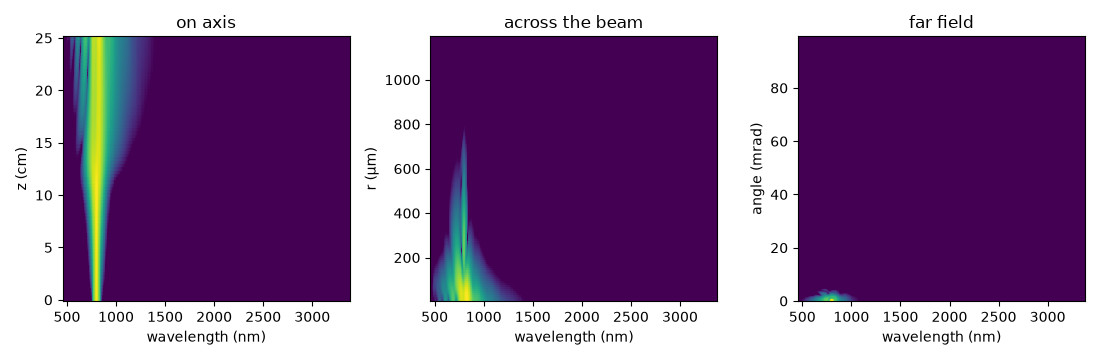
The spectrum on the axis, across the beam, and in the far field#
The on-axis spectrum broadens where the filament forms. At the last plane, the spectrum across the beam shows the core’s broadening, and the far field the rings of conical emission. Each has its own unit; the colours here are in dB of each.
x, on_axis = on_axis_spectra(result)
r, x_r, across = radial_spectrum(result)
theta, x_f, far = far_field(result)


def decibels(values):
    """Return values in dB below their largest, floored at -40 dB."""
    return 10 * np.log10(np.maximum(values / values.max(), 1e-4))


figure, axes = plt.subplots(1, 3, figsize=(11, 3.6))
z = np.asarray(result["z"]) * 100
axes[0].pcolormesh(x * 1e9, z, decibels(on_axis), shading="auto")
axes[0].set(xlabel="wavelength (nm)", ylabel="z (cm)", title="on axis")
axes[1].pcolormesh(x_r * 1e9, r * 1e6, decibels(np.maximum(across, 0)), shading="auto")
axes[1].set(xlabel="wavelength (nm)", ylabel="r (µm)", title="across the beam")
axes[2].pcolormesh(x_f * 1e9, theta * 1e3, decibels(far), shading="auto")
axes[2].set(xlabel="wavelength (nm)", ylabel="angle (mrad)", title="far field")
figure.tight_layout()
print(f"Complete filament reader example: {perf_counter() - started:.1f} s")
Complete filament reader example: 9.5 s