The desktop front end

solprop-gui is a desktop window for setting up, running and reading solprop simulations without writing a script. It is written for physicists who know the experiment they want to model: a setup is described in physics terms (a capillary’s core radius, a gas and its pressure, a pulse’s wavelength, duration and energy), and solprop’s own keyword names stay behind an Advanced section.

The front end is experimental. Its window, its workflow and the files it writes for itself may change between releases before 1.0; the recipes and results files it makes are solprop’s own, and keep solprop’s guarantees.

The window holds no physics of its own. Every number it shows, from a soliton order on the setup sheet to a pulse’s width on a results page, is computed by solprop; every setup it writes is a solprop recipe, which solprop run and Recipe.load read in the same way; and every run is an ordinary solprop results file that the processing functions read. What you build in the window can be continued in a script, and a script’s recipe can be opened in the window.

Installing and starting it

The front end is an extra of solprop, installed with it:

uv pip install "solprop[gui]"
solprop-gui

or, with pip, python -m pip install "solprop[gui]". It runs on the platforms of the installation page, with the native backend those wheels carry. From a checkout of the repository, add the extra to the environment and start the window without syncing it again:

uv sync --extra gui
uv run --no-sync solprop-gui

uv sync builds the native backend from native/ and needs a C++20 compiler; with no compiler, follow the lightweight setup of contributing and install the wheel CI built with uv run --no-sync poe fetch-wheel.

On Linux the window needs a few system libraries that Qt loads. On Debian or Ubuntu:

sudo apt install libegl1 libxkbcommon0 libxcb-cursor0

The window is drawn with Qt (PySide6) and pyqtgraph. Its publication figures are drawn with Matplotlib through solprop.plotting, so they match the figures a script makes.

The window

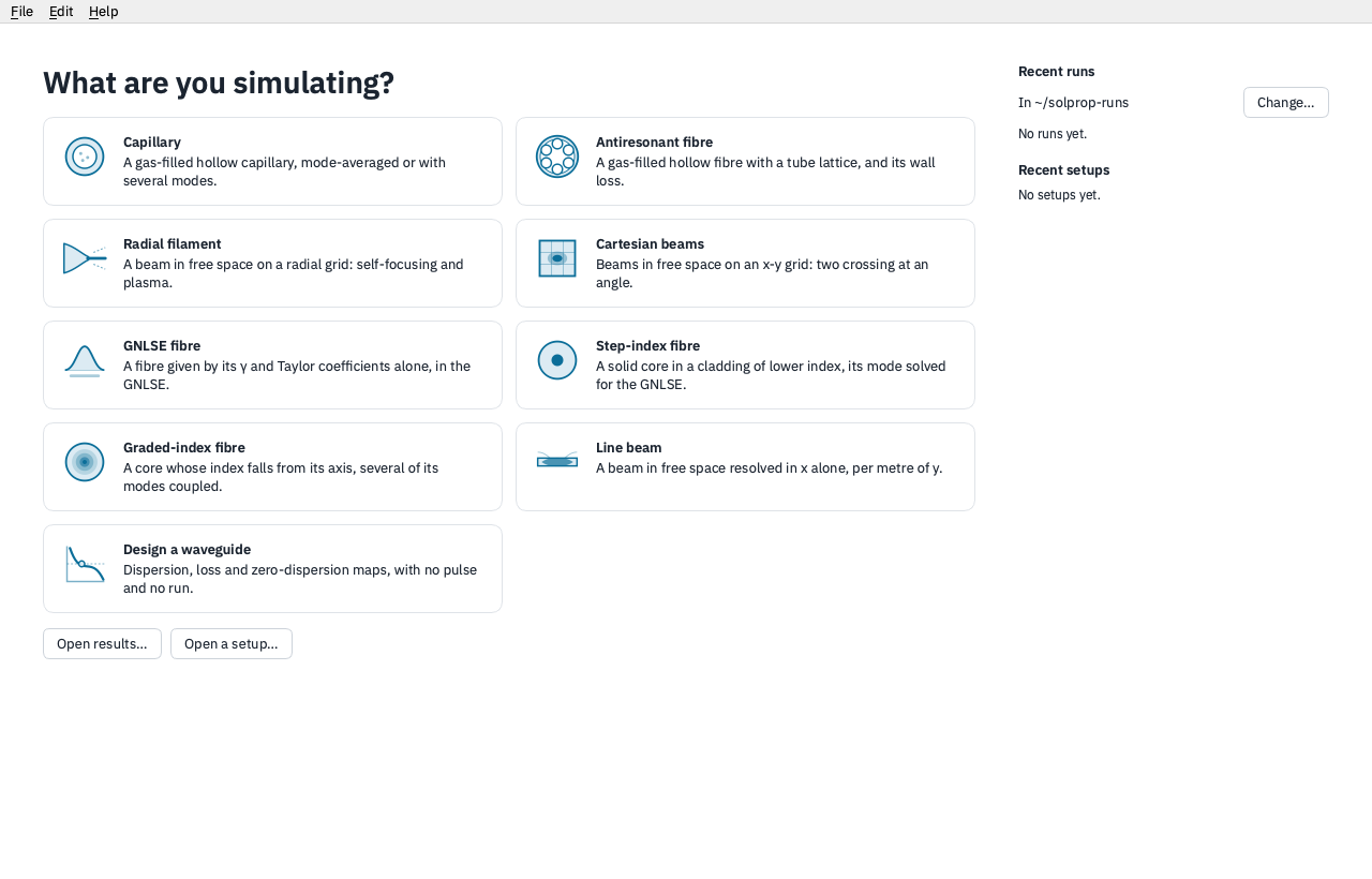
A bar across the top of the window names the stage you are on:

stage	what it is for
Home	Choose what to simulate, design a waveguide, or open a setup or a results file
Setup	One sheet of the setup’s parameters, with the numbers they give and a preview plot
Run	The run as it goes: its progress, and the spectrum and pulse growing along z
Analyse	Pages of the results, all at one position along z
Scan	A scan over one or more of the setup’s parameters, and its results

The button at the right of the bar does the stage’s main thing: Run on a setup, Stop while a run goes, Rerun afterwards, Run scan on the Scan stage and Simulate this when designing a waveguide. The ⋯ menu beside it saves the setup, shows it as a recipe, or shows it as the Python that builds it. File and Edit hold the same with their usual shortcuts; every change to a setup is one step of Undo. Help → User guide (F1 on Windows and Linux) opens this chapter in a window of its own; it comes with the front end, so it reads offline. Help → About solprop gives the versions running and the project’s links.

A run goes into a folder of its own, <date>-<title>, holding its results file run.h5, the recipe it ran (recipe.toml) and its log (run.log). The folders are made in ~/solprop-runs unless you choose another with Change… under Recent runs on Home; the window remembers the choice. The folder is the record: Home lists what it finds there, and copying a run’s folder elsewhere loses nothing.

In this chapter

• A first simulation follows one setup from Home to its results: a resonant dispersive wave in a helium-filled capillary.

• The problem classes describes what each tile on Home sets up, and the numbers and pages it has.

• Reading the results covers the Analyse pages, the plot tools and exporting.

• Scans runs a setup over a grid of its parameters.

• Designing a waveguide explores a guide’s dispersion, loss and phase matching with no pulse and no run.

• Running on other machines sends runs and scans to a workstation, a Slurm cluster or a rented machine over SSH, and lists every run on every machine.