Reading the results#
The Analyse stage is a rail of pages down the left and one page shown at a time. Every page is at the same position along z, chosen with the z slider at the foot of the window, and each page’s controls sit beside it on the right. A run’s own pages depend on its class (the problem classes); a page that a results file cannot support is shown greyed out, with the reason as its tooltip.
The pages read the results file through solprop.processing, the same functions
a script uses (reading results), so a number on a page is
the one a script gets. Opening a results file from Home brings back its setup too, from
the recipe the file records.
Moving through a run#
The z slider sets the plane every page shows. Clicking a map whose axis is z, or dragging along it, moves the plane to that point.
Left and right arrow keys step a plane; up and down step a page.
While a run goes, Follow the newest plane keeps the slider on the plane last saved.
The pages#
These are the guided classes’ pages; the free-space ones are in the problem classes.
Overview shows the spectrum and the pulse along z as maps, and both at the plane as lines. The spectral axis is wavelength or frequency, the spectra are in decibels down to a floor you set, and Time range sets how much of the window the pulse map shows.
At this plane gives the plane’s energy and duration, then its spectrum, its pulse and its spectral phase. Type a band or drag one on the spectrum: the page then gives the energy in the band, and draws the pulse filtered to it beside the whole pulse. Whole spectrum clears the band. With several modes, choose one mode or their sum.
Spectrogram is the plane’s spectrogram, gated by a pulse whose width you set
(solprop’s get_spectrogram()).
Along z plots what solprop recorded at every step, up to four quantities at once: energy, peak power and intensity, electron density and the others the run’s statistics hold. Log axes is Auto by default, which puts a quantity that spans decades on a logarithmic axis.
Modes, for a run of several modes, gives the energy in each mode along z and each mode’s spectrum at the plane.
Compress sends the plane through a chain of optical elements (chirped mirrors, a prism pair, a grating pair, a length of glass or gas, or a Taylor phase) and draws the pulse before, after and at its transform limit (compression). An element set to Auto is searched by solprop for the shortest pulse; Take the values found fixes them. The plane and band compressed are the ones chosen on At this plane.
Run health says how the run went: its step size along z with the rejected steps, the light removed at the time window’s edges, the run’s record (its backend, precision and threads, its wall time and peak memory) and its log. Check it before trusting a result: a run whose light reaches the window’s edges, or whose steps collapse, needs a wider window or a smaller tolerance (numerics).
The plot tools#
Every plot in the window works the same way.
Hover over a plot to read it: on a line plot, the nearest curve’s value under the pointer; on a map, the position and the value there.
Zoom with the wheel over the plot, or over one axis to zoom that axis alone. Drag to pan. A double click goes back to the page’s own view. A zoomed plot keeps its view while the plane changes or a run redraws it.
Right-click for what can be done at that point:
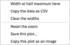
Width at half maximum here measures the width of the nearest curve’s peak at half its height (3 dB down on a decibel axis), and draws it on the curve with its value; Clear the widths takes the measurements away.
Copy the data as CSV puts the plot’s curves on the clipboard.
Go to the peak, on a map along z, moves the plane to where the map is highest.
Reset the zoom, Save this plot… (PNG, or SVG) and Copy this plot as an image.
Pulses are drawn four times finer than the run’s own time samples, by zero-padding
their spectrum as get_power() does with
oversampling=4: this adds no information, but draws a short pulse smoothly and finds
its peak between the samples.
Exporting#
Each page’s Export menu has:
Publication figure…, the page drawn by
solprop.plottingwith Matplotlib, as PDF, SVG or PNG. Maps in it are embedded as images, so a vector figure stays small. It is offered where solprop draws the page; a free-space run’s pages have none yet.This page as an image…, the page as it is on screen.
Data as CSV…, the page’s lines, where it has them.
Copy as Python, the code that draws the page from the results file with
solprop.processingandsolprop.plotting, to carry on in a script.